It is very important to validate the models before using them in any generation. Models are prone to making errors, and incorporating bad models adds noise to the system.
Machine learning and statistics are complex; in this article, we provide some explanations and tips to interpret the performance of the models and decide whether it makes sense to use them or not. If you want to have a quick overview, we advise you to take a look at this video: https://www.youtube.com/watch?v=4jRBRDbJemM
QSAR performance metrics
When Makya generates new molecules, those can be given prediction scores using QSAR models. For a given objective and a given molecule, the model outputs a probability between 0 and 1. Below 0.5 the molecule is considered as inactive on the objective, while above 0.5 the molecule is considered as active. This 0.5 threshold is used to perform the calculation of all the following metrics. This threshold can be reconsidered depending on the model performance and the expectation of the user.
To summarise:
AUC (Area Under the Curve)
The Area Under the Curve (AUC) is the measure of the ability of classifier to distinguish between classes, i.e. the greater the AUC, the better is the performance of the model in classifying data points between positive and negative classes. The AUC has a range between 0 and 1. Simply put, when AUC is equal to 1, the classifier is able to perfectly distinguish and classify points between the two classes. However, if the AUC is 0 then the classifier would make wrong predictions every single time. When AUC equals 0.5, the classifier either predicts a random class or a constant class for all data points, which is just as undesirable.
The AUC provides in a single number, a good idea of the performance of a model, regardless of the selected probability threshold.
NOTE: when the model is trained on an imbalanced dataset (having a lot more inactive than active compounds), the AUC can be strongly misleading, reaching high scores with poor classification abilities. In the case of an imbalanced dataset, we recommend considering the AUC PR and F1-score instead.
The shape of the FPRs vs FTRs curve (also called the ROC curve), on which the AUC is calculated, is also important. For example, when the curve starts vertically, this means that the rate of true positives is high while that of false positives is low, synonymous with an excellent model for high probabilities.
When a predictor for an important objective has disappointing performances, we recommend creating a new predictor for that objective with a relaxed threshold.
Confusion Matrix
The Confusion Matrix is used to illustrate classifier performances based on the four values: true positives (TP), true negatives (TN), false positives (FP) and false negatives (FN). They are plotted against each other to show a confusion matrix. In green we have good predictions, in red, bad ones.
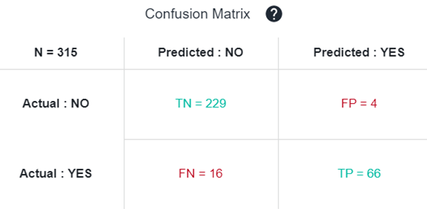
From this confusion matrix, several metrics such as Accuracy, Precision, Recall, and F1-score can be calculated to assess particular aspect of the model performance. Depending on the usage of the model, some are more important than others.
Accuracy
Accuracy describes the number of correct predictions (active/inactive) over all predictions. It is perhaps the most intuitive of the model evaluation metrics, and thus commonly used.
Accuracy = (TP + TN) / (TP + TN + FP + FN)
In Makya, the predictions of "inactive" are not very important since you are interested in active molecules usually, so another interesting metrics to consider is the precision.
Precision
Precision (or specificity) is a measure of how many of the positive predictions made are correct (true positives).
Precision = TP / (TP + FP)
In other words, a precision of 0.9 means that you have 90% chances to be active when the model predicts a molecule as active.
It is interesting to compare that metrics to the Normalized precision which is the percentage of active molecules in the training set. For instance if you have a precision of 50% you may think that the model is not really good, but if in the initial dataset you have only 10% of active compounds, the normalized precision will be 5, meaning that you have 5 times more chances to be active when using the model, which is actually not too bad.
Recall
Recall (or Sensitivity) is a measure of how many of the positive cases of the initial training set were correctly predicted, or caught as active, by the model.
Recall = TP / (TP + FN)
Indeed a model can have a very good precision but if most of the time it predicts the molecules as inactive in order to avoid making mistakes, then it becomes useless. This what recall assesses.
A simple analogy to understand precision and recall
To understand precision and recall even better, let us consider an analogy: you are fishing along a lake and throw a large net to catch fishes.
If you catch 7 out of 10 total fishes in the lake, then that's 70% recall (calling 70% of all fish) and 100% precision, because you caught only fishes. But if you were to capture 7 stones along with 7 fish, then that's only 50% precision (and still 70% recall) as half the items caught in the net are useless.
To avoid the junk stones, you could use a smaller net and and try to catch only fish in areas of high-fish and low-stones density. In this case you might catch only 3 fish and no rocks, and hence that gets you 30% recall and 100% precision.
The precision/recall trade-off
In an ideal world, our aim would always be to achieve a 100% precision and 100% recall.
Unfortunately, in the real world, we can't have both and attempts to increase precision will reduce recall, and vice versa. This is called the precision/recall trade-off.
In the analogy presented above, an attempt to increase precision is made by using a smaller net in higher fish-density regions of the lake. A caveat of this strategy is that a lower number of fish is caught, which corresponds to a lower recall.
Hence, if your main focus is to always predict carcinogenicity correctly, your model needs to have a high precision, in which case sometimes a safe compound will be predicted as carcinogenic (low recall).
F1-score
F1-score combines both precision and recall. The idea is to provide a single metric that weights the two ratios (precision and recall) in a balanced way, requiring both to have a higher value for the F1-score value to rise.
F1-score = 2 * (Precision * Recall) / (Precision + Recall)
NOTE: the F1-score is a better indicator of the actual performances of the model than the AUC when the training dataset is imbalanced. As such, it is a very informative metrics. However, it also gives as much weight to the recall as to the precision, while chemists are often more interested in the precision.
Having a look to the Precision/Recall vs Threshold curve allow you also to reconsider the probability threshold to define active vs inactive.
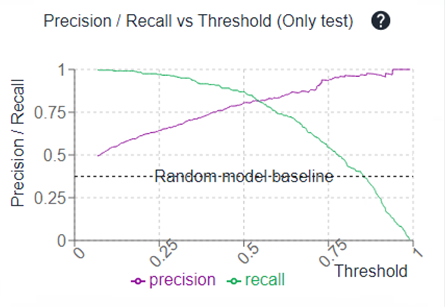
For instance, if you have a plateau where the precision is quite similar between 0.3 and 0.5 probability thresholds, maybe putting a cut at 0.3 (probability) is a good idea during your molecule selection since it will allow you to have more propositions because of a better recall, with very few impact on the precision.
Using a threshold different to 0.5
To put a cut at a certain probability threshold that is not 0.5 (for example, 0.3 in the example above), in the Parallel Coordinates of your generated molecules, you can filter molecules that have a predicted score above the threshold of interest. In the example described above, we would filter molecules with an prediction score above 0.3 on the predicted objective.
These molecules would not all be displayed in the IN BLUEPRINT selection, since some would have prediction scores below 0.5.